SCF Methods — Diagonalisation & Orbital Transformation
CP2K summer school 2018
Self Consistent Field (SCF)
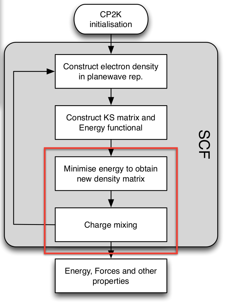
- Central to the QuickStep (DFT) calculation is the Self-Consistent-Field cycle \begin{align} H[\rho] \phi_n = E_n \phi_n\\ \rho(\mathbf{r}) = \sum_n f_n \phi^*_n(\mathbf{r}) \phi_n(\mathbf{r}) \end{align}
-
Key to speed and stability of the calculation:
- Energy minimisation
- Charge mixing
Overview
- Common Methods In CP2K
- Eigensolvers (diagonlisation)
- Charge Mixing for Diagonalisation Methods
- Optimisers
- Orbital Transformation (OT)
- Preconditioners
- Orbital Transformation (OT)
- Comparison of OT and Diagonalization.
- Eigensolvers (diagonlisation)
This talk is only an introductory overview.
A much more detailed version of this talk given by Lianheng Tong at the 2016 summer school.
Generalised Eigenvalue Problem
We converted the Kohn-Sham equations into matrix form by introducing basis functions.
\begin{align} \mathbf{H C} = \mathbf{E S C}\\ \end{align}
Where
- $\mathbf{H}$ is the matrix representation of the Kohn-Sham equations
- $\mathbf{C}$ is the matrix of Molecular Orbital coefficients of the basis functions used
- $\mathbf{S}$ is the overlap matrix showing how the basis functions overlap (are not orthogonal).
- $\mathbf{E}$ is the matrix with the eigenenergies of the MOs.
Eigenvalue Problem
change variables
\begin{align} \mathbf{H C} & = \mathbf{E S C}\\ \mathbf{H S^{-1/2} S^{1/2} C} & = \mathbf{E S^{1/2} S^{1/2} C}\\ \mathbf{S^{-1/2} H S^{-1/2} S^{1/2} C} & = \mathbf{S^{-1/2} E S^{1/2} S^{1/2} C}\\ \mathbf{S^{-1/2} H S^{-1/2} C'} & = \mathbf{E S^{-1/2} S^{1/2} C'}\\ \mathbf{H' C'} & = \mathbf{ E C'}\\ \end{align}
where $\mathbf{C'} = \mathbf{S}^{1/2} \mathbf{C}'$ and $\mathbf{H}' = \mathbf{S}^{-1/2} \mathbf{H} \mathbf{S}^{-1/2}$, is a standard (non-linear) Eigenvalue problem.
Diagonalisation
we can diagnonalise $\mathbf{H' C'} = \mathbf{ E C'}$ to find a new set of MOs given the input Kohn-Sham matrix built from the current density.
Standard methods of diagonalising the matrix can be used - termed 'traditional diagonalisation'.
The new orbitals are used to build
- a new density
- a new Kohn-Sham matrix
Then the process repeats until (if?) it converges - i.e. MOs in are the same as MOs out.
Charge density mixing
Instead of using the new set of orbitals directly mix together some older solutions and the new solution.
Much more stable that blindly taking only the new density.
In the simplest case linearly mix $\alpha$ of the new density with $1-\alpha$ of the density in the previous step.
Input - linear mixing
&SCF
   SCF_GUESS ATOMIC
   EPS_SCF 1.0E-06
   MAX_SCF 50
   &MIXING
       ALPHA 0.2 !sensible value, the default 0.4 is very aggressive.
   &END MIXING
&END SCF
Instead of mixing in a fraction of the new density with the previous step a more sophisticated approach mixes in a history of previous density using some 'recipe'.
By default CP2K switches to the DIIS method when the largest change in an element of the density matrix is smaller than EPS_DIIS, which is 0.05 by if not set explicitly.
Output
should look something like this:
 Step  Update method          Time   Convergence      Total energy         Change
 ---------------------------------------------------------------------------------
 1     P_Mix/Diag. 0.50E+00    2.1   0.41056021     -2133.4408435676     -2.13E+03
 2     P_Mix/Diag. 0.50E+00    3.2   0.20432922     -2132.0776002852      1.36E+00
 3     P_Mix/Diag. 0.50E+00    3.2   0.10741372     -2131.3677551799      7.10E-01
 4     P_Mix/Diag. 0.50E+00    3.2   0.05420394     -2131.0080867703      3.60E-01
 5     DIIS/Diag.  0.39E-03    3.2   0.02722180     -2130.8276990683      1.80E-01
 6     DIIS/Diag.  0.19E-03    3.1   0.00062404     -2130.6473761946      1.80E-01
 7     DIIS/Diag.  0.84E-04    3.2   0.00050993     -2130.6473778175     -1.62E-06
note the switch to DIIS when Convergence is < 0.05.
Smearing
For metallic systems we generalise how we build the density. Up to now we build the density by filling the $N$ electrons into the $N$ lowest molecular spin orbitals.
Problem
If the system is metallic (or has a very small band-gap) this can lead to 'charge sloshing'. The orbitals around the 'fermi energy' can change their ordering, and different ones are occupied from iteration to iteration.
Solution
Fill the orbitals using a Fermi-Dirac distribution at a fictitious finite temperature - smooths out charge sloshing.
Smearing input
&SCF
   SCF_GUESS ATOMIC
   EPS_SCF 1.0E-6
   MAX_SCF 50
   ADDED_MOS 200
   &SMEAR ON
       METHOD FERMI_DIRAC
       ELECTRONIC_TEMPERATURE [K] 300
   &END SMEAR
   &MIXING
       METHOD BRYODEN_MIXING
       ALPHA 0.2
       NBUFFER 5
   &END MIXING
&END SCF
We also use a different mixing scheme, which is probably optimal for metallic systems.
Fermi Temperature is typically between 300 - 3000 K. The larger the value the smoother convergence, but it can affect the physical properties of the system if too large.
OT
why not just directly minimize the energy functional with respect to the MO coefficients?
- we need our orbitals to remain orthogonal - Pauli principle
So the minimization must be subject to a constraint - on an M dimensional hypersphere!

This is built into diagonalisation, as the new vectors are always eigenfunctions of the (current) Kohn-Sham matrix.
change variables in some clever way that builds in the constraint
Work with new variables $\mathbf{X}$
$$\mathbf{C}(\mathbf{X}) = \mathbf{C}_0 \cos(\mathbf{U}) + \mathbf{X U}^{-1} \sin(\mathbf{U})$$
$$\mathbf{U} = (\mathbf{X}^T\mathbf{SX})^{1/2}$$

Can show that this leads to optimization in an M-1 dimensional linear space.
Change variables in some clever way that builds in the constraint.

We can use standard minimization routines and we never have to diagonalise the Kohn-Sham matrix!
Far more robust - but requires a band gap - revert to diagonalization and smearing for metallic systems.
Preconditioning
In minimization problems it is often a good idea change the problem by applying some approximate solution to the problem to make an equivalent set of equations that are
- approximately diagonal
- with diagonal elements of the same size and of order 1.
The OT solver is no exception. There are a variety of preconditioners available, and they can dramatically speed up convergence.
OT recipe 1 - small-medium systems
&SCF
    SCF_GUESS RESTART
    EPS_SCF 1.0E-06
    MAX_SCF 20
    &OT ON
        MINIMIZER DIIS
        PRECONDITIONER FULL_ALL
        ENERGY_GAP 0.001
    &END OT
    &OUTER_SCF
        MAX_SCF 2
    &END OUTER_SCF
&END SCF
This uses the most efficient minimizer, DIIS. Change to CG for difficult systems.
The most accurate, and expensive to calculate, preconditioner -
FULL_ALL.The
OUTER_SCFrestarts the SCF cycle and reapplies a new preconditioner when the original loop finishes.
OT recipe 2 - pretty large systems
&SCF
    SCF_GUESS RESTART
    EPS_SCF 1.0E-06
    MAX_SCF 20
    &OT ON
        MINIMIZER DIIS
        PRECONDITIONER FULL_SINGLE_INVERSE
        ENERGY_GAP 0.1
    &END OT
    &OUTER_SCF
        MAX_SCF 2
    &END OUTER_SCF
&END SCF
The FULL_ALL preconditioner is expensive to apply to large systems (diagonalization of the approximate Hamiltonian is required). The FULL_SINGLE_INVERSE is pretty good, and much cheaper for big systems.
Choice of method
- Use OT if you can, it is faster and converges more reliably
- disadvantage: requires additional calculations to obtain unoccupied states.
- Use Diagonalisation if you need to work with the occupation numbers of orbitals
- Use Diagonalisation (with smearing) for metallic systems
The two methods use quite different code paths.
EPS_SCFhas different meanings for OT (largest derivative of energy wrt MO coefficients) and TD (largest change in the density matrix).
Some options will only work with either OT or TD.
- Most common is
MOsection inPRINTonly works properly with diagonalisation MO_CUBESsection inPRINTonly works properly with OT.
Summary
See a more detailed version of this talk given by Lianheng Tong at the 2016 summer school, if you want to know (much) more!